When working with a large data set, you would be more productive if you knew how to quickly find what you need. Luckily, Excel has a few functions that can help with this.
1FIND
The FIND Function in Excel returns the numerical position of a specified character or string (sequence of characters) within a larger string. It’s useful for precise text extraction, manipulation, and conditional formatting.
The syntax for the FIND function is:
FIND(search_text, text_to_search_in, [start_position])Here, search_text is the character or substring you want to locate, and text_to_search_in is the larger text string you want to search. The start_position parameter specifies where you want the function to begin searching in the string.
Any parameter in square brackets is optional.
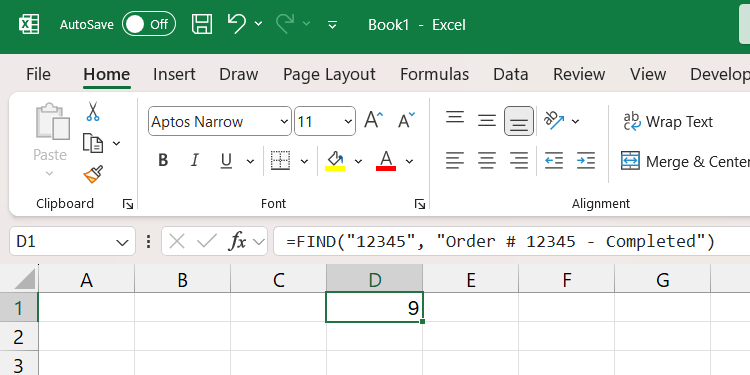
Here is an example of how the FIND function would look in action:
=FIND("12345", "Order # 12345 - Completed")The above formula will return 9, since the substring 12345 starts at that position.
The FIND function is case-sensitive. It distinguishes between uppercase and lowercase letters. If, for instance, you searched for the letter A in the substring apples, you would get an error.
If you want to find something while ignoring case sensitivity, use the SEARCH function instead. It has a similar syntax to the FIND function.
=SEARCH(search_text, text_to_search_in, [start_position])2SORT
The SORT function can help if you need to arrange data in a range in ascending or descending order to make it easier to find specific data in your Excel sheet.
The syntax of the SORT function is:
SORT(range_to_sort, [sort_index], [sort_order], [sort_by])The range_to_sort parameter is the range you want to sort. Use the sort_index parameter to specify which column or row number to sort by within the range (default is 1).
The sort_order parameter specifies the order for sorting the list, where 1 is ascending and -1 is descending (default is ascending). And sort_by specifies whether to sort by rows (FALSE), which is the default, or columns (TRUE).
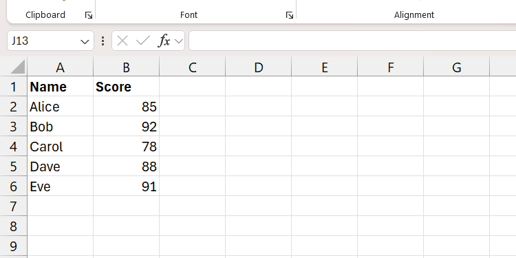
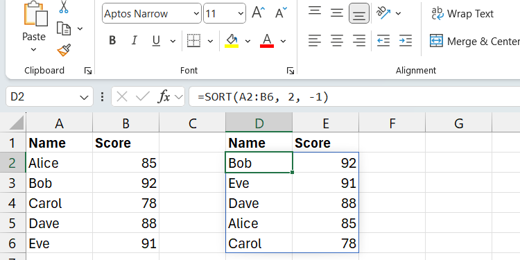
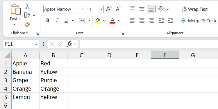
We are going to sort the range in the screenshot below based on the second column and in descending order.
Here is what the formula would look like in Excel:
=SORT(A2:B6, 2, -1)The range should now be sorted in descending order.
3FILTER
The FILTER function evaluates a range of data based on a condition and returns only the rows and columns that meet the condition.
The syntax of the FILTER function is:
FILTER(range_to_filter, condition, [value_if_empty])The range_to_filter parameter is the array or range of cells you want to filter. The condition parameter is the criteria that determines what should be returned in the filtered result. The value_if_empty parameter specifies what should be returned if nothing satisfies the condition.
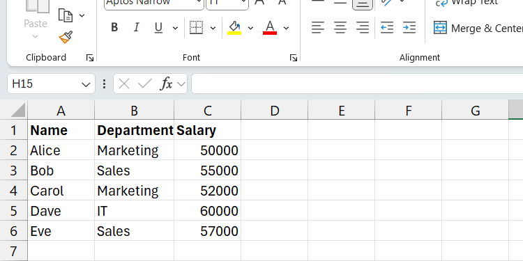
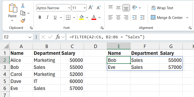
We will filter the range in the screenshot below to show only employees in the Sales department.
Here is what the formula looks like in action:
=FILTER(A2:C6, B2:B6 = "Sales")You should now only see the rows and columns that meet the specified criteria.
4INDEX
If you want to get the value of a particular cell in a data range, you can use the INDEX function. You just need to specify the row and column where it’s located.
The syntax of the INDEX function is:
INDEX(range_to_search, row_to_search_in, [column_to_search_in])The range_to_search parameter is the range from which you’ll retrieve the value. The row_to_search_in and column_to_search_in are the row and column numbers where the value is located within the range (think of them as coordinates).
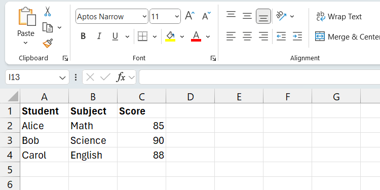
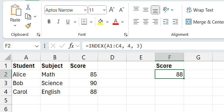
For instance, in the screenshot below, we’ll retrieve the Score (C4) that Alice got in her English test.
Here is what the formula looks like:
=INDEX(A1:C4, 4, 3)This formula will return 88 since that is what Alice scored on her English test.
5MATCH
The MATCH function in Excel searches a range of data for a specified value and then returns its relative position. You can then use the returned value with functions like INDEX to retrieve and manipulate data dynamically.
The syntax of the MATCH function is:
MATCH(value_to_search, range_to_search_in, [match_type])Here, value_to_search is the value you want to find and range_to_search_in is the range where you are searching for it.
The match_type parameter specifies the type of match to use. Here are the types you can use:
| Match Type | Description |
|---|---|
| 1 (default) | Return the largest value less than or equal to value_to_search |
| 0 | Return an exact match |
| -1 | Return the smallest value greater than or equal to value_to_search |
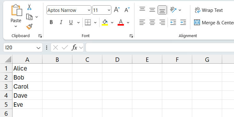
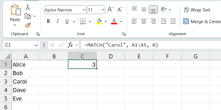
For our example, we’ll use the MATCH function to find the position of Carol in the range. We also want it to be an exact match.
Here is what the function would look like in Excel:
=MATCH("Carol", A2:A6, 0)After running the formula above, the function will return 3 since the exact match of Carol is the third item in the range.
6XLOOKUP
With the XLOOKUP function, you specify a value to search for in a range and then extract the corresponding value from another range. Unlike the HLOOKUP function and VLOOKUP function, XLOOKUP allows you to search in any direction, making looking up data in your sheet more flexible.
The syntax of the XLOOKUP function is:
XLOOKUP(value_to_look_up, range_to_check, range_to_return, [if_value_not_found], [match_type], [search_mode])In this syntax, the value_to_look_up is the value you are looking up, range_to_check is the range where the value you want will be extracted, and range_to_return is where the corresponding value of the lookup value will come from. You only need to specify these three parameters for the function to work, so these are the only ones we will focus on.
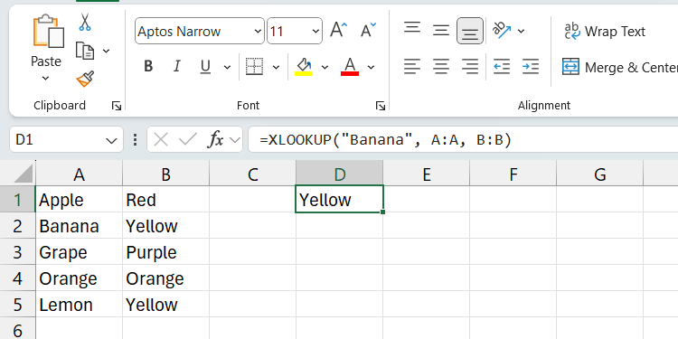
Let’s clear this up with an example based on the screenshot below. We want to look up Banana (A2) and return its color from the corresponding column (B).
Here is what the formula will look like in Excel:
=XLOOKUP("Banana", A:A, B:B)Running this will return Yellow (B2), the corresponding value based on looking up the value Banana.
Mastering these six Excel functions—FIND, SORT, FILTER, INDEX, MATCH, and XLOOKUP—will help you quickly locate, organize, and extract information from large datasets. This can significantly improve your Excel productivity and ability to analyze data efficiently.

