Key Takeaways
- Cell references in Excel are like addresses that point to specific cells.
- Three types of Excel cell references are relative, absolute, and mixed, each with unique functions.
- Mastering cell references is crucial for creating flexible spreadsheets, making tasks like budgeting and data analysis much easier and more efficient.
Cell references are at the core of how Microsoft Excel operates. Whether you’re working with simple calculations or complex formulas, understanding cell references and mastering the different types of references is key to getting accurate results.
What Are Cell References in Excel?
A cell reference is simply a way of identifying a specific cell in your spreadsheet.
Every Excel worksheet has several rows and columns, with cells (boxes) in each row and column. As you work, you’ll input values or text into these cells. In the first row, you’ll find letters, which are used to name the columns. Then, in the first column, you’ll find numbers, which are used to name the rows.
To identify a cell, you only need to identify the naming letter and number. For instance, the cell in the second column and row is A1 (the letter always precedes the number) by default. A1, in this instance, is a cell reference.
When you use a cell reference in a formula, you can easily reference the data in that cell. You don’t need to copy and paste values each time you need to use a calculation operator.
For instance, if you’re performing the SUM function for cells A1 to A5 [=SUM(A1:A5)], your calculations will always adjust automatically when data in the cells changes. As long as the value in the cell changes, the result of the operation would change since you’re referencing the cell, not the value in the cell.
Cell references make it possible to build flexible spreadsheets that easily adapt to data changes. This is particularly useful for tasks like budgeting, data analysis, and reporting, where data can change frequently.
There are three types of cell references in Microsoft Excel.
- Relative reference
- Absolute reference
- Mixed reference, which is basically just a blend of relative and absolute references
Each type of cell reference differs in terms of how you want Microsoft Excel to treat the referenced cell when you copy or move formulas.
Relative Cell References
By default, cell references in Microsoft Excel are relative. Remember that a cell reference is basically a cell address, like how you get to the cell (e.g., A2). When you use A2 in a formula, it’s a reference relative to the row and column. If you move the formula to another row or column, the reference changes in relation to the cell in the new row or column.
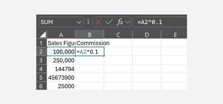
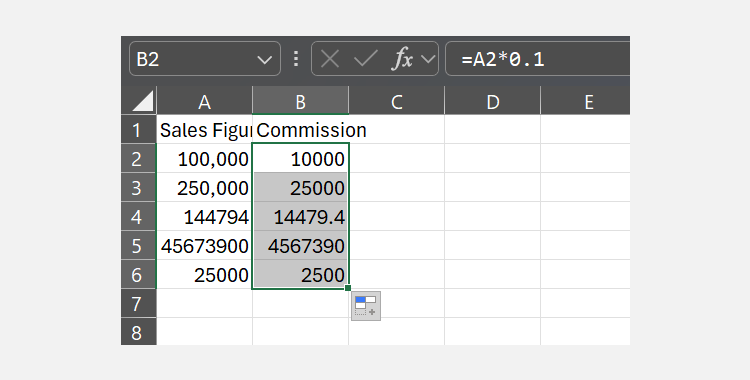
Imagine you have a list of sales figures in column A, and you want to insert a 10% commission in column B for each sales figure. You can use the formula [=A2*0.1] in cell B2 and drag the formula down the entire B column.
Excel will automatically adjust the references to A3, A4, and so on.
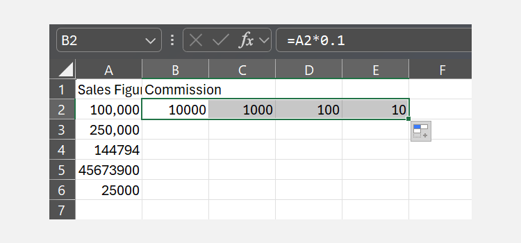
If you extend the formula to the right instead, the reference will change in relation to the new location. Instead of A2 in the formula [=A2*0.1], Excel will automatically adjust the references to B2, C2, and so on.
Basically, if you copy a formula containing one cell reference (e.g., [=A2+B2]) from one cell (e.g., C2) and paste it into another cell (e.g., C3), Excel will shift the reference based on the new location of the formula. So, the formula will change from [=A2+B2] to [=A3+B3] in the new cell (C3).
This is especially useful when you want to perform the same function across many rows or columns without manually adjusting the formula.
Absolute Cell References
This type of cell reference stays fixed no matter where you move the formula. It’s best for when you want a formula to always refer to the same cell, regardless of where it’s used.
An absolute reference is denoted by a dollar sign ($) before both the column and row number (e.g., $A$2). If you only place one dollar sign, either before the column or the row, it’ll be a mixed reference. For instance, $A2 fixes only the column, while A$2 fixes only the row. However, $A$2 fixes the row and column. No matter where you move the formula, the reference will always point to cell A2.
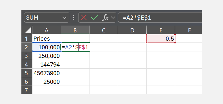
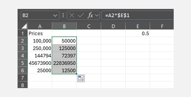
Suppose you have a fixed tax rate in cell E1 and a list of prices in column A. To calculate the tax for each price, you could use the formula [=A2*$E$1] in cell B2.
The dollar signs ensure that every formula in column B will always reference D1 for the tax rate, even when you drag the formula down. The reference to A2 will change when you copy the formula down, but the reference to $E$1 will remain fixed.
Without this absolute reference, Excel would reference cells E2, E3, etc., which wouldn’t give the correct results.
Absolute cell references are perfect when you’re working with constants—values that do not change, like tax rates, interest rates, or any fixed value you want to apply consistently across your data.
Mixed Cell References
A mixed cell reference is a blend consisting of a relative and absolute reference. Remember that every cell reference has two parts—the row and the column aspect of the cell. In a mixed cell reference, one part would be relative and the other absolute. That is, the column could be fixed while the row would be relative, or vice versa.
As in the example above, $A2 fixes the column and keeps the row relative, while A$2 fixes the row and keeps the column relative.
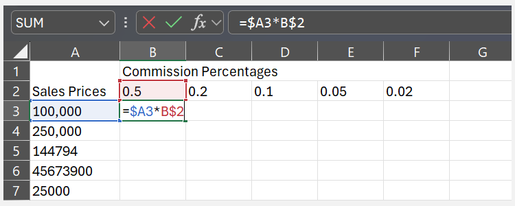
Suppose you want to obtain different percentages of different sales figures in Excel. For your row headers, you can place the sales figures. Then, you place the commission percentages as your column headers. The goal for each cell is to multiply its corresponding row value by the column value.
In the first cell (in my case, B3), you can use this formula:
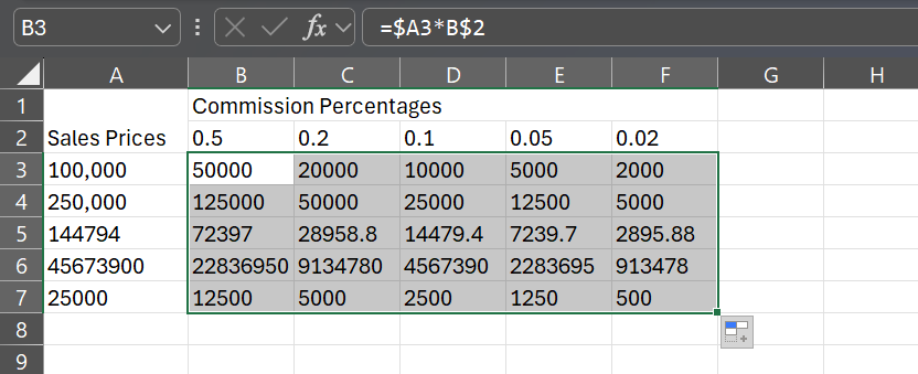
=$A3*B$2For the first part of the formula, column A is fixed. This way, when you copy the formula across columns, it will always refer to the values in column A. However, the row number, which isn’t fixed, will always change based on the row the formula is copied to.
For the second part of the formula, row 2 is fixed. As a result, when you copy the formula down rows, it will always refer to the values in row 2. However, the column letter, which isn’t fixed, will adjust depending on the column the formula is copied to.
If you click Formulas > Show Formulas, you can see how the formula has changed across the cells.
With mixed cell references, you can maintain a consistent reference point for either a row or column while allowing the other to change.
